
This independent project analysed Scottish GDP growth using a wide range of macroeconomic indicators and compared multiple modelling approaches to both understand the drivers of GDP growth and the challenges of forecasting it. The analysis drew together drew together both internal (domestic) and external (international) economic indicators which were then transformed into growth based measures. Four approaches were used in modelling: a full multiple regression model, a reduced regression model, a lagged regression model, and benchmark forecasting models using ARIMA and a simple machine learning model, decision trees.
The results suggested that output per job growth is the most consistent and statistically significant explanatoy factor across the regression models, while retail growth and Brent oil price growth also show explanatory value in specific model specifications. The full regression model achieved a relatively strong fit, with an adjusted R-squared of 0.72 whereas the lagged model also performed well, yielindg an adjust R-squared of 0.67. Regression diagnostics indicated no major issues with multicollinearity, heteroskedasticity or position autocorrelation in the main models.
That being said, the decision tree model performed substantially worse out of sample than in sample with a negative test R-squared, indicating overfitting and weak generalisation. This suggests that although non-linear models can identify patterns in the training data, they struggle with small macroeconomic datasets and structural breaks. And therein lies one of the significant limitations faced in modelling here – limited historical data, dating back to 1998 and with yearly data sets, this led to around 25 data points (from 1998 to 2023).
The ARIMA model provided a useful benchmark by modelling GDP growth based only on its own past values, allowing comparison between purely time-series dynamics and models that incorporate explanatory variables.
Overall, the project demonstrated that Scottish GDP growth can be analysed meaningfully using structured statistical methods but forecasting performance is constrained by limited data, structural shocks, and the inherent volatility of macroeconomic relationships.
The project therefore highlights not only the value of modelling, but also the importance of sound economic judgement, careful data preparation, and critical interpretation when using data to support decisions.
1.Introduction
The purpose of this independent project was to analyse and model the drivers of Scottish GDP Growth using a set of macroeconomic indicators that aim to capture a wide range of economic conditions such as: labour market prices, domestic demand, productivity, energy market exposure, and external market conditions. GDP growth is one of the most important indidcators of economic performance (or lack there of) and understanding its drivers is crucial to fiscal planning, economic forecasting, and policy development.
Rather than relying on a single model, the project was designed to compare multiple approaches. This was important for two reasons: Firstly, because GDP growth is influenced by several (both measurable and immeasurable) overlapping economic forces, so it’s useful to examine the explanatory contribution of different economic indicators. Secondly, because forecasting macroeconomic indicators is inherently difficult as these indicators are essentially all driven by human behaviour at all levels (ordinary citizens, governments, policymakers, investment banks, hedge funds, etc), and by trying to predict such variables we are essentially aiming to predict human behaviour, which is quite difficult – so it becomes essential to compare multiple models to provide a balanced view of what the data can and cannot explain, and to interpret what it can explain with sound judgement.
The analysis therefore focused on three related questions:
- Which indicators appear to be associated with GDP growth?
- How stable and interpretable are those relationsihps under different model specifications?
- How well do different modelling approaches perform when using to predict GDP growth?
2.Data Collection and Preparation
2.1Data Sources
The analysis combined both UK wide and Scottish economic indicators with externally sourced commodity price and exchange rate data. The core dataset included the following variables:
- Scottish GDP Growth Rate
- Scottish Unemployment Rate
- UK CPI Inflation Rate
- Scottish Average annual earnings for full-time employees
- Scottish Retail sales growth rate
- Scottish economic output per job
- Scottish total Scottish annual oil and gas production
- Brent crude oil price
- GBP/EUR Exchange Rate
Facing data limitations, I could not find the Scottish annual CPI inflation rate, so the UK one was utilised.
Brent crude oil prices were utilised due to Scotland’s heavy reliance on imported oil, as well as it’s drilling operations in the North Sea impacting economic activity . The GBP/EUR exchange rate was utilised as the European Union is the UK’s largest trading partner, and based on my thought process, exchange rates are likely influence the level of trade between the two countries. Both brent crude oil prices and the GBP/EUR exchange rates, were extracted externally from the Federal Economic Reserve (FRED) using built in APIs in R.
The other Scottish indicators were drawn from prepared template files from government-based websites: Office for National Statistics and the Scottish Government.
This multi-source and multi-variate approach was vital because GDP growth is not driven be one dimension alone. Labour market conditions, domestic activity, productivity, energy prices, exchanges rates and many others, can all either directly or indirectly through deeper cause and effect relationships, either positively or negatively impact GDP.
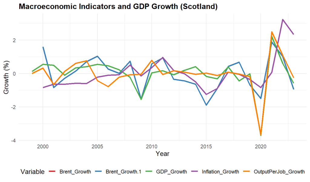
A plot of all growth rate variables excluding Output per Job Growth, Earnings per Job Growth, and Exchange rate Growth can be seen below.
2.2Data merging and cleaning
The datasets were merged by calendar year to create a unified modelling dataset. This required:
- converting date fields into numeric year values
- renaming and aligning variables across sources
- removing unmatched observations
- excluding rows with missing values after lag creation or growth rate calculations
Some datasets had observations up to 2025, others only up to 2023, so all datasets were unified from 1998 to 2023.
2.3Variable Transformation
A key methodological decision was to transform several variables into growth rates rather than using their raw levels. This was done to reduce the influence of long-term trends and better capture the meaningful year to year economic changes.
The following transformations were applied:
- Inflation growth from CPI
- Earnings growth from annual earnings
- Oil and gas production growth
- Brent price growth
- Exchange-rate growth
Unemployment rate growth, retail growth and output-per-job growth were already expressed in a suitable form for analysis.
This step was important because macroeconomic time series often trend over time and modelling raw levels can create misleading relationships driven purely by upward (or downward) movement rather than actual explanatory power.
2.4 Lagged variables
A third regression model was constructed using lagged version of selected variables, this included:
- lagged unemployment
- lagged inflation
- lagged retail activity
- lagged Brent growth
This step was taken to reflect the economic reality that many indicators affect GDP with an inherent delay rather instead of instantaneously, like a series of dominos falling in but on a much larger and complex scale. Lagged variables therefore provide a more realistic structure of economic activity for forecasting and consequently, interpretation.
3. Methodology
The project used five modelling approaches:
- Full multiple linear regression
- Simple two-variable regression
- Reduced multiple regression
- Lagged multiple regression
- Decision tree regression
- ARIMA time-series model
Although the main focus was on four methods, the regression work included multiple specifications in order to test stability and improve interpretation.
3.1 Full multiple linear regression
The first model used all main macroeconomic indicators:
- unemployment rate
- inflation growth
- earnings growth
- retail growth
- oil and gas growth
- output per job growth
- Brent growth
- FX growth
This model simply aimed to identify which combination of domestic and external indicators best explained GDP growth.
3.2 Simple regression model
A very limited model using only unemployment and inflation growth was estimated as a comparison case. This provided a useful baseline as to whether a small set of commonly referenced macro indicators could explain GDP growth by themselves or not.
3.3 Reduced regression model
A second multiple regression specification was estimated using a narrower set of indicators:
- unemployment rate
- inflation growth
- retail growth
- Brent growth
- FX growth
This reduced model was designed to improve interpretability and assess whether a more focused set of demand and external indicators could explain GDP growth without the full complexity of the larger model with 8 predictors.
3.4 Lagged regression model
The lagged model introduced delayed versions of selected predictors whilst retaining some structural variables such as earnings growth, oil and gas growth, output per job growth, and FX growth. This model was intended to reflect more realistic economic timing and test whether delayed explanatory effects improved model quality.
3.5 Decision tree regression
A decision tree model was built using the same macroeconomic features. Unlike linear regression, a decision tree does not assume linear relationships. Instead, it recursively splits the data into smaller groups based on threshold rules in the predictors.
This method was included for two reasons:
- to test whether GDP growth responds to macro variables in a non-linear way
- to compare a machine learning model against more traditional econometric approaches
The model was evaluated using train/test performance metrics, including RMSE, MAE, and R-squared.
3.6 ARIMA model
A univariate ARIMA model was estimated using GDP growth alone. This served as a benchmark model, allowing comparison between:
- models that use explanatory macroeconomic variables
- a model that relies only on the historical behaviour of GDP growth itself
Doing this was useful in assessing whether GDP growth could be forecast more effectively from its own internal time-series structure than from the selected external predictors. It allows us to question whether its even worth it to spend so much time and resources building models, when GDP can simply be forecast from it’s own values.
4. Regression Results
4.1 Full multiple regression model
The full model produced the following key results:
- Multiple R-squared: 0.820
- Adjusted R-squared: 0.724
- F-statistic p-value: 0.000218
This suggests a strong overall in sample fit with the model explaining a substantial proportion of the variation in GDP growth.
Significant variables
Two variables were statistically significant:
- Retail growth: coefficient = 0.472, p = 0.0387
- Output per job growth: coefficient = 0.771, p = 0.000382
Interpretation
These results suggest that:
- stronger retail performance is associated with higher GDP growth,, which is consistent with the role of domestic demand
- growth in output per job, a productivity-related measure, is strongly associated with GDP growth, suggesting that productivity is a central driver of economic expansion
Other variables such as unemployment, inflation, oil and gas growth, Brent growth, earnings growth, and FX growth, were not statistically significant in this specification. This does not necessarily mean they are irrelevant economically, it’s just that within this sample and model structure, their independent explanatory contribution is not estimated precisely.
4.2 Simple unemployment and inflation model
The simplified model using only unemployment and inflation growth performed poorly:
- R-squared: 0.020
- Adjusted R-squared: -0.073
- F-statistic p-value: 0.805
No variable was significant here.
Interpretation
This result is quite useful, not disappointing. It shows us that unemployment and inflation alone do not explain Scottish GDP growth well over this sample. That suggests growth dynamics are broader and more dependent on productivity demand and external factors than can be captured solely by these two variables in isolation.
This is an important analytical finding because it demonstrates that a plausible but overly simple model may be insufficient for real-world economic analysis and forecasting.
4.3 Reduced regression model
The reduced model produced:
- Multiple R-squared: 0.461
- Adjusted R-squared: 0.311
- F-statistic p-value: 0.0353
Within this model, Brent growth was statistically significant:
- coefficient = 0.078
- p = 0.0026
Interpretation
This suggests that external energy price conditions may have a measurable relationship with Scottish GDP growth, which is plausible given Scotland’s exposure to energy-related activity. However, the model explains substantially less variation than the full model, which indicates that excluding productivity and some broader activity variables reduces explanatory power.
4.4 Lagged regression model
The lagged model produced:
- Multiple R-squared: 0.790
- Adjusted R-squared: 0.670
- F-statistic p-value: 0.00117
Again, Output per job growth was highly significant:
- coefficient = 0.832
- p = 7.33e-05
The lagged unemployment, inflation, retail and Brent variables were not individually significant, but the model as a whole remained statistically significant.
Interpretation
This result is important for two reasons.
Firstly, the lagged structure is more realistic than a purely contemporaneous model, because macroeconomic variables often affect GDP with a delay.
Secondly, the continued significance of output-per-job growth suggests that productivity-related dynamics remain the most robust explanatory factor across different model specifications.
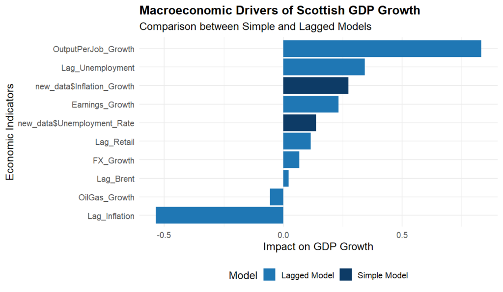
This makes the lagged model quite valuable for the report because it combines stronger economic realism with relatively strong explanatory performance. Both models can overall show strong explanatory performance and the results of such can be seen below.
5. Regression Diagnostics
A range of diagnostic checks were carried out to test whether the regression assumptions were broadly satisfied.
5.1 Multicollinearity
Variance Inflation Factors for the full model were all relatively low:
- unemployment: 1.74
- inflation: 3.27
- earnings: 1.53
- retail: 2.65
- oil and gas: 2.09
- output per job: 2.20
- Brent: 2.06
- FX: 1.10
Interpretation
These values do not indicate severe multicollinearity. While some predictors are naturally related, the model does not appear to suffer from the degree of predictor overlap that would invalidate the regression.
5.2 Heteroskedasticity
Breusch–Pagan tests were not statistically significant for the estimated models:
- full model p-value: 0.551
- reduced model p-value: 0.527
Interpretation
There is no strong evidence that residual variance changes systematically with fitted values. This suggests the homoskedasticity assumption is broadly reasonable.
5.3 Autocorrelation
Durbin–Watson test results were:
- full model DW = 2.14, p = 0.434
- reduced model DW = 2.53, p = 0.823
Interpretation
These values do not suggest problematic positive autocorrelation in the residuals. That is quite encouraging, especially given that this is a time-series dataset.
6. Decision Tree Results
The decision tree model was used to test whether non-linear threshold effects in the data could improve predictive performance relative to linear regression.
I created two versions of the decision tree in Python with varying tree depths, both with similar performance patterns.
Decision tree performance (1st version)
- Train RMSE: 1.084
- Test RMSE: 7.567
- Train MAE: 0.821
- Test MAE: 5.447
- Train R-squared: 0.640
- Test R-squared: -0.098
Decision tree performance (2nd version)
- Train RMSE: 1.096
- Test RMSE: 7.412
- Train MAE: 0.838
- Test MAE: 6.060
- Train R-squared: 0.632
- Test R-squared: -0.053
Interpretation
These results show a clear pattern:
- the model performs reasonably well on the training data
- performance deteriorates sharply on the test data
- test R-squared is negative in both cases
A negative test R-squared means that the model performs worse than simply predicting the average GDP growth value for all test observations. This indicates poor generalisation.
What this means
The decision tree appeared to be overfitting the training data. In other words, it is learning patterns that do not hold up well when applied to unseen observations.
This is not a failure of the project. On the contrary, it is an important analytical finding. It suggests that:
- the dataset is too small for a tree-based model to generalise well
- macroeconomic relationships may not be stable enough for this kind of split-based model at annual frequency
- non-linear models can fit noise rather than signal when data are limited
Why this is valuable
Including the decision tree strengthens the project because it demonstrates that alternative and more complex modelling approaches were tested rather than assumed to be superior. The result provides evidence that, in this case, a machine learning approach is less suitable than the more interpretable econometric models.
7. ARIMA Results
The ARIMA model was estimated as a univariate benchmark using GDP growth alone.
The role of the ARIMA model in this project is not necessarily to outperform all other approaches, but to answer a specific question:
How much of GDP growth can be forecast from its own past behaviour, without using explanatory macroeconomic indicators?
Interpretation
If ARIMA performs comparably to the regression models, that suggests GDP growth has meaningful internal time-series structure and that the selected indicators add limited forecasting value. If it performs worse, it suggests that explanatory variables do provide useful information beyond GDP’s own past.
Even without emphasising a single headline metric, the inclusion of ARIMA is valuable because it shows awareness of the difference between:
- explanatory modelling
- predictive time-series modelling
This broadens the methodological strength of the project.
8. Key Analytical Findings
Across the different models, several findings emerged.
8.1 Productivity appears to be the strongest and most consistent driver
Output-per-job growth is highly significant in both the full and lagged regressions. This suggests that productivity-related dynamics are central to understanding Scottish GDP growth in this dataset.
8.2 Domestic demand matters
Retail growth is significant in the full model, indicating that stronger consumer related activity is associated with higher GDP growth. This makes sense given that Scotland (and the UK as a whole) is a service based economy with limted manufacturing.
8.3 External energy conditions matter, but not consistently across all specifications
Brent growth is significant in the reduced model, suggesting that global energy prices may influence Scottish growth. However, its effect is less robust when the model includes a broader set of variables.
8.4 Simple macro stories are insufficient
A model using only unemployment and inflation explains almost none of the variation in GDP growth. This highlights the importance of using a broader and more structured set of indicators.
8.5 Model form matters
The decision tree performed poorly out of sample, while the regression models remained more interpretable and statistically coherent. This suggests that for small annual macroeconomic datasets, transparent models may be more informative than highly flexible ones.
9. Limitations
This anakysis comes with several important limitations.
9.1 Small sample size
The analysis uses annual data over a relatively limited number of observations. This reduces statistical power and makes all models more sensitive to unusual years.
9.2 Structural shocks
Macroeconomic relationships are affected by major disruptions, including financial crises and pandemic related shocks. These events can weaken model stability and reduce predictive accuracy. Termed “Black swan events”, by Nassim Nicholas Taleb, these are rare, unpredictable and high impact events which defy conventional forecasting models, often resulting in severe economic consquences and losses.
9.3 Potential overlap in economic variables
Some variables, especially output-per-job growth and GDP growth, are closely related economically. This makes interpretation important and means coefficients should not be treated as pure causal effects.
9.4 Forecasting difficulty
The weak out of sample performance of the decision tree model shows that forecasting GDP is substantially harder than fitting relationships in sample. This is a real world limitation, not simply a technical one.
9.5 Annual frequency
Annual data may obscure shorter-term economic dynamics that would be more visible in quarterly data, and possibly more helpful in modelling and forecasting.
10. Conclusion
This project used a structured analytical approach to examine Scottish GDP growth using multiple data sources and multiple modelling methods. The process involved collecting and merging economic and market data, transforming variables into economically meaningful growth measures, testing different model specifications, conducting regression diagnostics, and comparing econometric and machine learning approaches.
The strongest overall conclusion is that productivity-related growth, measured here through output per job growth, is the most consistent explanatory factor in the dataset, while retail growth and external energy conditions also appear relevant in some specifications. At the same time, the analysis shows that GDP forecasting is difficult, especially when using limited annual data and when structural shocks affect the economy.
From an analytical perspective, the value of the project lies not only in which variables appear significant, but also in the methodological judgement it demonstrates:
- selecting and preparing data from multiple sources
- transforming variables appropriately
- comparing models rather than relying on one approach
- testing assumptions and diagnostics
- identifying limitations and interpreting results cautiously
Overall, the project shows how data analysis, statistical modelling, and critical interpretation can be used together to support economic understanding and inform decision-making, while also recognising the limits of forecasting in a complex macroeconomic environment.
The policy implications of this model are discussed in the next report.